From Complexity to Clarity: Simplifying Principal Component Analysis (PCA)

 

"Principal Component Analysis (PCA) is by far the most popular dimensionality reduction algorithm. It is a statistical procedure which is also used for finding patterns in high dimension data. It uses an orthogonal transformation to convert a set of observations of possibly correlated variables into a set of values of linearly uncorrelated variables called as principal components."

I know after reading the above paragraph you are like... 

Oh, really? Why it couldn’t possibly be any easier? 

Then answer is... well, of course, it is simple! and, don’t stress—I’m here to save the day, because clearly, that’s what was missing all along

Principal Component Analysis: Because Your Data Has Too Many Opinions, Just Like Your Ex Used To 🤭

Lets forget you ex and discuss the agenda, what all things we are going to cover in this article?

1.) What even is PCA?

2.) Why PCA? or, "Why Shrink Your Data?"

3.) How does PCA actually works?

4.) Application of PCA (Yes people actually use it)

5.) Math Stuff

6.) Python Coding Example

7.) Conclusion: Do you really need it?

1. What Even Is PCA?

* Definition: Principal Component Analysis — or, as we like to call it, "Magic Math that Makes Your Data Less Annoying."
* Simple Explanation: It’s where we take a perfectly fine dataset, perform a mathy shuffle dance, and end up with fewer columns that apparently contain the same enough information. Simple, right?
* Behind the Scenes: Eigenvalues, eigenvectors, matrices… you know, all the good stuff you happily forgot after that one linear algebra class.

2. Why PCA? Or, "Why Shrink Your Data?"

* To Stop Crashing Your Laptop: Imagine actually trying to work with a 100-dimensional dataset. PCA helps avoid the horror of infinite loading circles.
* Because Interpretability Is for Amateurs: With PCA, you can have the thrill of knowing your data just got simpler without needing to explain why.
* Optimal Confusion Guarantee: Impress your friends and baffle your audience with reduced dimensions that convey almost the same story. Who doesn’t love a good riddle in data form?

3. How Does PCA Actually Work?

* Step-by-Step Guide: A 15-step process of complex calculations, conveniently glossed over in most blog posts. But don’t worry — you can just use a library function! I have covered that in 6 steps.
* Scaling Your Data Like a Pro: Normalize first, or you’ll end up with results that don’t make sense (not that they ever really do).
* Covariance and Variance Fun: Rejoice in knowing how much variation you can squeeze out of your data without it screaming back in protest.

4. Applications of PCA (Yes, People Actually Use It)

* Dimensionality Reduction (Obviously): Because who needs all those columns when you can turn them into just a few "principal components"? Image Compression, a.k.a. “Why’s My Picture Blurry Now?” Ever wonder how to shrink images into an indecipherable mosaic? PCA’s got you covered.
* Pattern Recognition and ML Models: You’ll get to say you improved your model’s performance by 0.02% and act like it’s groundbreaking.
* Noise Reduction (Or Data Disguising): PCA will kindly help you ignore all the pesky little outliers you didn't want to deal with.

5. Math Stuff

This section is for nerds, who are interested in the math behind this algorithm. 

Steps to perform PCA:

(i) Standardize the dataset.
(ii) Calculate the covariance matrix for the feature in data.
(iii) Calculate the eigen values and eigen vectors for covariance matrix.
(iv) Sort eigen values and their corresponding eigen vectors.
(v) Pick k eigen values and form a matrix of eigen vector.
(vi) Transform original matrix.

(i) Standardize the dataset.

Let's assume we have data with 4 features & 5 rows of training data

Training Data Table

Feature 1	Feature 2	Feature 3	Feature 4
1	2	3	4
5	5	6	7
1	4	2	3
5	3	2	1
8	1	2	2

Standardize the data : 

Where:

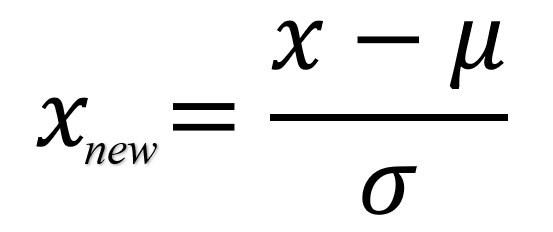
• $z$z: The standardized value (z-score).
• $x$x: The original data point.
• $\mu$μ: The mean of the dataset.
• $\sigma$σ: The standard deviation of the dataset.

 

	Feature 1	Feature 2	Feature 3	Feature 4
μ =	4	3	3	3.4
σ =	3	1.58	1.73	2.30

(Standardize Data) Apply formula in each feature:

Feature 1	Feature 2	Feature 3	Feature 4
-1	-0.63	0	0.26
0.33	1.26	1.73	1.56
-1	0.63	-0.57	-0.17
0.33	0	-0.57	-1.06
1.33	-1.26	-0.57	-0.60

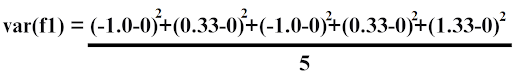
(ii) Calculate the covariance matrix for the feature in data.

For Population:

For Sample:

Calculate covariance matrix of given data.

	Feature 1	Feature 2	Feature 3	Feature 4
Feature 1	var(f1)	cov(f1,f2)	cov(f1,f3)	cov(f1,f4)
Feature 2	cov(f2,f1)	var(f2)	cov(f2,f3)	cov(f2,f4)
Feature 3	cov(f3,f1)	cov(f3,f2)	var(f2)	cov(f3,f4)
Feature 4	cov(f4,f1)	cov(f4,f2)	cov(f4,f3)	var(f4)

μ of each feature is 1 & σ is 0. Since we are standardizing.

Var(f1) = 0.8

Cov(f1,f2) = -0.2529

- Like this calculation the other covariance is:

	Feature 1	Feature 2	Feature 3	Feature 4
Feature 1	0.8	-0.25	0.03	-0.14
Feature 2	-0.25	0.8	0.51	0.49
Feature 3	0.03	0.51	0.8	0.75
Feature 4	-0.14	0.49	0.75	0.8

(iii) Calculate the eigen values and eigen vectors for covariance matrix.

- A eigen vector is an non-zero vector that changes at most by a scalar factor when that linear transformation is applied to it.

- The corresponding eigen value is the factor by which the eigen vector is scaled.

- Let 'A' be a square matrix (in our case the covariance matrix), 'v' a vector & 'λ' a scalar that satisfies Av = λv , then λ is called eigen value associated with eigen vector v of A.

Rearranging the above equation:

Av - λv = 0; (A-λ1)v = 0

Since we know v is non-zero, only way this equation can be equal to 0, if

det(A-λ1)=0

	Feature 1	Feature 2	Feature 3	Feature 4
Feature 1	0.8-λ	-0.25	0.03	-0.14
Feature 2	-0.25	0.8-λ	0.51	0.49
Feature 3	0.03	0.51	0.8-λ	0.75
Feature 4	-0.14	0.49	0.75	0.8-λ

Solving the above equation = 0

Eigen Vectors:

solving the (A-λI)v = 0 equation for vector with the different λ values:

0.8-λ	-0.25	0.03	-0.14
-0.25	0.8-λ	0.51	0.49
0.03	0.51	0.8-λ	0.75
-0.14	0.49	0.75	0.8-λ

x

v1

v2

v3

v4

= 0

for λ = 2.51, solving the above equation using Cramer's rule, the values for vectors "v" are 

v₁ = 0.16

v₂ = -0.52

v₃ = -0.58

v₄ = -0.59

 

Going by the same approach we can calculate the eigen vectors for the other eigen values.

We can form matrix using eigen vectors.

e1	e2	e3	e4
0.16	-0.91	-0.30	0.19
-0.52	0.20	-0.81	0.12
-0.58	-0.32	0.18	-0.72
-0.59	-0.11	0.44	0.65

(iv) Sort eigen values & their corresponding eigen vectors

Since eigen values are already sorted so no need to sort them again.

(v) Pick eigen values and from matrix of eigen vectors

If we choose the top 2 eigen vectors, the matrix will look like this

(Top 2 eigen vectors 4 * 2 matrix)

e1	e2
0.16	-0.91
-0.52	0.20
-0.58	-0.32
-0.59	-0.11

(vi) Transform the original matrix

Feature_matrix * Top_k_eigen_vectors = Transformed_data

Feature 1	Feature 2	Feature 3	Feature 4
-1.00	-0.63	0.00	0.26
0.33	1.26	1.73	1.56
-1.00	0.63	-0.57	-0.17
0.33	0.00	-0.57	-1.04
1.33	-1.26	-0.57	-0.60

x

e1	e2
0.16	-0.91
-0.52	0.20
-0.58	-0.32
-0.59	-0.11

=

nf1	nf2
0.01	0.75
-2.55	-0.78
-0.05	1.25
1.01	0.00
1.57	-1.22

6. Python Coding Example

# Code Example:

import pandas as pd
import numpy as np

# Input data
A = np.matrix([[1, 2, 3, 4], [5, 5, 6, 7], [1, 4, 2, 3], [5, 3, 2, 1], [8, 1, 2, 2]])

# Create DataFrame
df = pd.DataFrame(A, columns=["f1", "f2", "f3", "f4"])

# Standardize the data
df_std = (df - df.mean()) / df.std()

# Number of Principal Components
n_components = 2

# Apply PCA
from sklearn.decomposition import PCA
pca = PCA(n_components=n_components)
pc = pca.fit_transform(df_std)

# Convert PCA results to DataFrame
principalDf = pd.DataFrame(data=pc, columns=["nf" + str(i + 1) for i in range(n_components)])

# Display output
print(principalDf)

Output

Index	nf1	nf2
0	-0.014003	-0.755975
1	2.556534	0.780432
2	0.051480	-1.253135
3	-1.014150	-0.000239
4	-1.579861	1.228917

7. Conclusion: Do You Really Need PCA?

Probably not, but it sure sounds fancy when you tell people at parties, right? If you love mysterious statistical transformations, you’re going to adore PCA!

I hope this helped you. If it did then please share it with your friends and spread this knowledge. 

Follow us at :

Instagram : 

https://www.instagram.com/infinitycode_x/


Facebook :

https://www.facebook.com/InfinitycodeX/


Twitter :

https://twitter.com/InfinityCodeX1